Budget Surplus or Deficit

Data

This plot uses the budget data frame of the gcubed package. In particular, the columns Year and SurpDef_pg are used. SurpDef_pg represents the surplus/deficit as a percentage of the US GDP for the given year. Some rows of the data frame are shown below.

The source of this data was the Federal Reserve Economic Data (FRED) of the St. Louis Fed.

library(gcubed)
budget[budget$Year %in% c(1970, 1980, 1990, 2000, 2010),
       c("Year", "SurpDef_pg")]

## # A tibble: 5 x 2
##    Year SurpDef_pg
##   <dbl>      <dbl>
## 1  1970       -0.3
## 2  1980       -2.6
## 3  1990       -3.7
## 4  2000        2.3
## 5  2010       -8.7

Code

First, we make a plot using geom_line. geom_hline is also used to create the x-axis.

library(ggplot2)
df <- budget[budget$Year >= 1950, ]

budget_plt <- ggplot(data = df, aes(x = Year, y = SurpDef_pg)) + 
  geom_line() + 
  geom_hline(yintercept = 0) + #deficit ribbon below
  theme_bw() +  
  ylab("Surplus or Deficit (% of GDP)") + 
  ggtitle("US Federal Budget (1950 - 2018) ") + 
    theme(panel.grid.minor = element_blank(), 
        axis.text.x = element_text(angle = 90), 
        plot.title = element_text(size = 20, face = "bold", hjust = 0.5),
        legend.title = element_blank())

budget_plt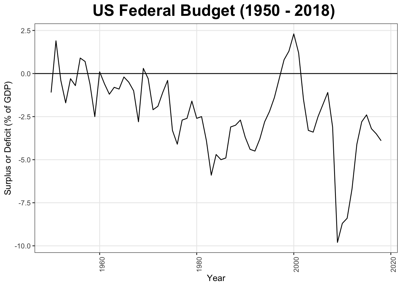 

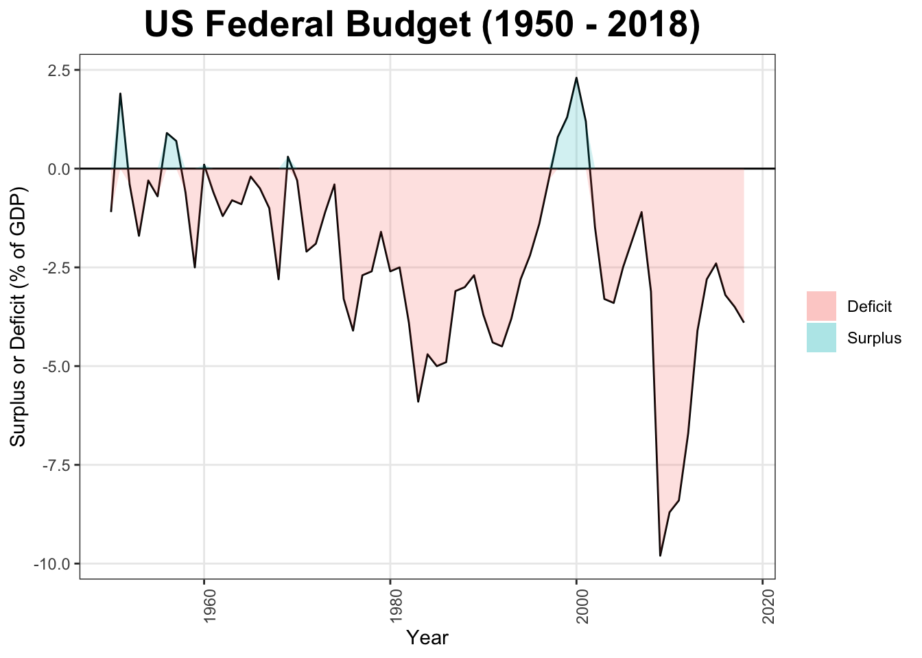
The filled-in regions are added using the geom_ribbon geometry.

budget_plt <- budget_plt + 
  geom_ribbon(aes(ymin = ifelse(SurpDef_pg < 0, SurpDef_pg, 0), 
                  ymax = 0, 
                  fill = "Deficit"), alpha = 0.2) +
  geom_ribbon(aes(ymin = 0,
                  ymax = ifelse(SurpDef_pg > 0, SurpDef_pg, 0), 
                  fill = "Surplus"), alpha = 0.2) 
  

budget_plt

Alternatively, all the code for the entire plot is shown below.

library(ggplot2)
library(gcubed)

df <- budget[budget$Year >= 1950, ]

budget_plt <- ggplot(data = df, aes(x = Year, y = SurpDef_pg)) + 
  geom_line() + 
  geom_hline(yintercept = 0) + #deficit ribbon below
  theme_bw() +  
  ylab("Surplus or Deficit (% of GDP)") + 
  ggtitle("US Federal Budget (1950 - 2018) ") + 
    theme(panel.grid.minor = element_blank(), 
        axis.text.x = element_text(angle = 90), 
        plot.title = element_text(size = 20, face = "bold", hjust = 0.5),
        legend.title = element_blank()) + 
  geom_ribbon(aes(ymin = ifelse(SurpDef_pg < 0, SurpDef_pg, 0), 
                  ymax = 0, 
                  fill = "Deficit"), alpha = 0.2) +
  geom_ribbon(aes(ymin = 0,
                  ymax = ifelse(SurpDef_pg > 0, SurpDef_pg, 0), 
                  fill = "Surplus"), alpha = 0.2)